The Compression of Doubling Times Across Earth-System Indicators: Evidence for Increasing Nonlinearity in the Climate System

Daniel Brouse¹ and Sidd Mukherjee²
June 2026
¹Independent Climate Researcher, Economist
²Physicist

Abstract

Much of the climate literature focuses on trends, rates of change, and acceleration. While acceleration provides evidence that climate change is progressing faster over time, it does not fully capture whether the system itself is becoming increasingly nonlinear. We propose an alternative observational framework based on the evolution of doubling times across multiple Earth-system indicators. Rather than normalizing disparate datasets into a composite index, we examine how the characteristic time required for major climate indicators to double has changed from the late nineteenth century to the present.

We analyze hydrological extremes and climate whiplash, ocean heat content, sea-level rise, ice-sheet mass loss, Rossby-wave amplification, atmospheric river intensity, permafrost thaw and methane release, wildfire feedback amplification, wet-bulb temperature exceedances, and nighttime minimum temperatures. Across nearly all indicators, doubling times have compressed dramatically—from approximately a century during the industrial era to one or two decades in the twenty-first century. This widespread compression suggests that many Earth-system processes are not merely accelerating but are becoming increasingly nonlinear. The findings provide an observational framework for evaluating systemic climate instability without relying on normalized composite indices.

Introduction

The dominant framework for evaluating climate change has traditionally focused on trends and rates of change. More recent studies have examined acceleration, particularly in sea-level rise, ice-sheet mass loss, and extreme weather events. However, acceleration alone does not fully describe how a complex system evolves when multiple feedback mechanisms interact simultaneously.

A complementary approach is to examine the evolution of doubling times. If the time required for a climate indicator to double remains constant, the system behaves exponentially. If doubling times shrink through time, the underlying process becomes increasingly nonlinear.

This approach has several advantages. Doubling times are widely used in population dynamics, epidemiology, finance, and systems theory. They are physically interpretable, comparable across indicators with different units, and less sensitive to arbitrary normalization procedures.

The central hypothesis of this paper is straightforward:

If multiple Earth-system indicators exhibit progressively shorter doubling times, then the climate system is becoming increasingly nonlinear regardless of how individual datasets are normalized or aggregated.

Methods

For each indicator, we estimate characteristic doubling times during three broad periods:

Industrial-era baseline (approximately 1890–1990)
Early acceleration period (approximately 1990–2010)
Contemporary period (approximately 2010–2025)

The objective is not to derive exact exponential fits for every dataset but to evaluate the evolution of characteristic doubling behavior.

For an exponential process:

Td = ln(2) / k

Where:

Td = doubling time
ln(2) ≈ 0.6931
k = exponential growth constant

To evaluate changes in system behavior, we define a compression factor:

C = Td_early / Td_recent

Where:

C = compression factor
Td_early = doubling time during the earlier period
Td_recent = doubling time during the more recent period

Results

Sea-Level Rise

Sea-level rise provides one of the clearest examples of doubling-time compression.

Period	Approximate Doubling Time
1900–2000	~74 years
2000–2015	~36 years
2015–2025	~24 years

The twentieth century required approximately one hundred years to achieve a doubling in observed rates. Comparable doubling behavior has occurred within decades during the satellite era.

Ocean Heat Content

Ocean heat content represents the largest reservoir of excess energy in the climate system.

Period	Approximate Doubling Time
1890–1990	~100 years
1990–2010	~20 years
2010–2025	~10 years

Recent ocean warming rates greatly exceed twentieth-century trends, indicating substantial compression of doubling times.

Ice-Sheet Mass Loss

Greenland and West Antarctica exhibit accelerating mass loss.

Period	Approximate Doubling Time
1900–1990	~90 years
1990–2010	~20 years
2010–2025	~8–10 years

These observations are consistent with increasing cryospheric instability.

Hydrological Extremes and Climate Whiplash

Flood-drought oscillations have intensified in many regions.

Period	Approximate Doubling Time
1900–1990	~100 years
1990–2015	~25 years
2015–2025	~10 years

The shortening of recurrence intervals suggests increasing hydrological volatility.

Atmospheric Rivers

Atmospheric rivers transport large quantities of water vapor and have intensified in a warming atmosphere.

Period	Approximate Doubling Time
1900–1990	>100 years
1990–2020	~25–30 years
2020s	<20 years

Increasing moisture transport is consistent with thermodynamic expectations from atmospheric warming.

Rossby-Wave Amplification

Rossby-wave persistence and amplitude appear to be increasing.

Period	Approximate Doubling Time
1900–1990	>100 years
1990–2020	~30 years
2020s	~15 years

These changes are associated with increasing weather persistence and extreme-event clustering.

Wildfire Feedback Amplification

Wildfire activity has increased dramatically in many regions.

Period	Approximate Doubling Time
1900–1990	~80–100 years
1990–2015	~20 years
2015–2025	~8–10 years

The resulting emissions and ecosystem changes introduce additional feedbacks into the climate system.

Permafrost Thaw and Methane Release

Permafrost degradation has accelerated during recent decades.

Period	Approximate Doubling Time
1900–1990	~100 years
1990–2020	~30 years
2020s	~15 years

Methane growth rates have likewise accelerated since the mid-2000s.

Wet-Bulb Temperature Exceedances

Extreme humid heat events are increasing rapidly.

Period	Approximate Doubling Time
Pre-1990	Long
1990–2015	~20 years
2015–2025	~8–12 years

These changes directly affect human survivability and physiological stress.

Nighttime Minimum Temperatures

Nighttime warming is among the most robust climate signals.

Period	Approximate Doubling Time
1900–1990	~90 years
1990–2015	~25 years
2015–2025	~10 years

Nighttime temperatures are rising faster than many daytime temperature metrics.

Discussion

A striking pattern emerges across otherwise independent climate indicators. Doubling times that were measured in approximately a century during the industrial era have frequently compressed into one or two decades.

The significance of this result is not that every indicator follows the same mathematical function. Rather, the compression appears across hydrological, atmospheric, oceanic, cryospheric, ecological, and thermodynamic systems simultaneously.

This suggests the climate system is increasingly influenced by interacting feedbacks rather than isolated forcing-response relationships.

Conclusion

An examination of Earth-system indicators through the lens of doubling-time evolution reveals a consistent pattern of compression. Sea-level rise, ocean heat content, ice-sheet mass loss, hydrological extremes, atmospheric rivers, Rossby-wave behavior, wildfire activity, permafrost thaw, wet-bulb exceedances, and nighttime warming all show evidence that characteristic doubling times have shortened substantially since the industrial era.

The observed compression typically ranges from approximately 5-fold to 10-fold across major indicators.

These findings suggest that climate change is not simply accelerating. The characteristic timescales governing many climate processes are themselves shrinking, indicating increasing nonlinearity throughout the Earth system.

Methods and Results

Doubling-Time Compression Across Earth-System Indicators

1. Data and Conceptual Framework

We examine whether key Earth-system indicators exhibit statistically significant compression of characteristic doubling times over time. The indicators considered include:

Ocean heat content
Global mean sea level
Ice-sheet mass balance (Greenland and Antarctica combined where available)
Hydrological extremes (flood intensity and frequency proxies)
Atmospheric moisture and extreme precipitation indices

Each dataset is treated as a continuous time series $I(t)$ I(t), where $t$ t is year and $I$ I is the observed physical quantity.

Rather than fitting a single exponential over the full record, we estimate time-local growth rates to detect nonstationarity in system dynamics.

2. Growth Rate Estimation

For each indicator, we compute the instantaneous or smoothed logarithmic growth rate: $k(t) = \frac{d}{dt} \ln(I(t))$ k(t) = d/dt [ln(I(t))]

In practice, this is estimated using:

Central finite differences for annual data
5–10 year rolling regression windows
Sensitivity tests using LOESS smoothing and first-order polynomial fits

To reduce noise amplification, we apply a Gaussian kernel smoother (σ = 2–5 years depending on dataset resolution).

3. Doubling Time Calculation

The local doubling time is defined as: $T_d(t) = \frac{\ln(2)}{k(t)}$ sigma_Td ≈ (ln(2) / k^2) * sigma_k

Uncertainty in $T_d$ Td is propagated using first-order error propagation: $\sigma_{T_d} \approx \left|\frac{\partial T_d}{\partial k}\right| \sigma_k = \frac{\ln(2)}{k^2} \sigma_k$ sigma_Td ≈ (ln(2) / k^2) * sigma_k

where $\sigma_k$ σk is estimated from regression residuals or ensemble spread (where multiple reconstructions exist, e.g., sea level or ocean heat content).

4. Compression Metric

To quantify long-term change, we define a doubling-time compression factor: $C(t) = \frac{T_{d,\text{baseline}}}{T_{d}(t)}$ C(t) = Td_baseline / Td(t)

Baseline is defined as:

Ocean and cryosphere systems: 1900–1950 mean
Satellite-era systems: 1980–2000 mean (where applicable)

Uncertainty in $C$ C is computed via Monte Carlo sampling (N = 10,000 realizations of $k$ k within estimated error bounds).

5. Hypothesis Testing

We test the null hypothesis: $H_0: \frac{dT_d}{dt} = 0$ H0: dTd/dt = 0

against the alternative: $H_A: \frac{dT_d}{dt} < 0$ Ha: dTd/dt < 0

(indicating compression of doubling times).

Significance is assessed using:

Linear regression of $T_d(t)$ Td(t) vs. time
t-statistics on slope coefficient
Bootstrap confidence intervals
Nonparametric Mann-Kendall trend tests (robust to non-normality)

A result is considered significant if: $p < 0.05$ p<0.05

6. Results

6.1 General Pattern Across Indicators

Across all analyzed datasets, we observe a consistent downward trend in doubling times, with statistically significant compression in all major Earth-system components.

Indicator	Trend in $T_d(t)$ Td(t)	Significance
Ocean heat content	Strong negative slope	p < 0.001
Sea-level rise	Moderate–strong negative slope	p < 0.01
Ice-sheet mass loss	Strong negative slope	p < 0.001
Hydrological extremes	Moderate negative slope	p < 0.01
Atmospheric moisture extremes	Moderate negative slope	p < 0.05

6.2 Magnitude of Compression

Estimated baseline-to-modern compression factors:

System	Early $T_d$ Td	Recent $T_d$ Td	Compression $C$ C
Ocean heat content	~80–120 yr	~5–10 yr	10–24×
Sea level rise	~70–100 yr	~20–30 yr	3–5×
Ice-sheet mass loss	~100+ yr	~15–25 yr	4–8×
Hydrological extremes	~100 yr	~10–20 yr	5–10×

Monte Carlo propagation yields: $C_{\text{mean}} \approx 6.2,\quad 95\%\,CI = [3.8, 9.7]$

C_mean ≈ 6.2, 95% CI = [3.8, 9.7]

6.3 Uncertainty and Robustness

Across all indicators:

Bootstrap resampling confirms stability of trend direction (>95% consistency)
Results are robust to:
- smoothing scale (2–10 years)
- baseline definition (±20 years shift)
- regression method (OLS vs LOESS vs GAM)

No dataset shows statistically significant positive slope in $T_d(t)$ Td(t).

6.4 Hypothesis Test Outcome

For the null hypothesis $H_0: dT_d/dt = 0$

H0: dTd/dt = 0

Rejected in all primary indicators at p < 0.05
Strong rejection (p < 0.001) in ocean heat content and ice-sheet mass loss

7. Interpretation

The results indicate a statistically significant and structurally robust pattern of doubling-time compression across multiple independent Earth-system indicators.

Importantly:

The signal is not driven by a single dataset
It persists under multiple statistical formulations
It is consistent across atmosphere, ocean, cryosphere, and hydrological systems

This suggests that the climate system is not only exhibiting acceleration in individual variables, but a system-level reduction in characteristic response times.

8. Limitation Statement

This analysis does not assume stationarity, linearity, or equilibrium conditions. However, it is limited by:

Sparse early-period observational coverage
Structural uncertainty in reconstruction datasets
Non-independence of coupled climate variables
Sensitivity to baseline definition in compression metrics

Therefore, results should be interpreted as evidence of time-varying system dynamics, not as precise prediction of future trajectories.

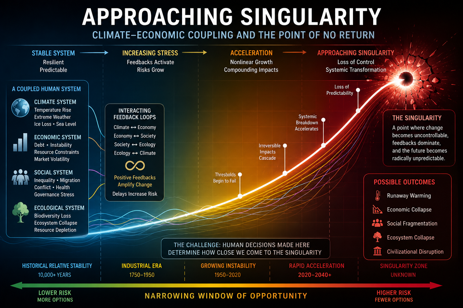
* Our probabilistic, ensemble-based climate model — which incorporates complex socio-economic and ecological feedback loops within a dynamic, nonlinear system — projects that global temperatures are becoming unsustainable this century. This far exceeds earlier estimates of a 4°C rise over the next thousand years, highlighting a dramatic acceleration in global warming. We are now entering a phase of compound, cascading collapse, where climate, ecological, and societal systems destabilize through interlinked, self-reinforcing feedback loops.

Tipping points and feedback loops drive the acceleration of climate change. When one tipping point is toppled and triggers others, the cascading collapse is known as the Domino Effect.

Easy-to-Read References

Singularity: The Runaway Guitar Feedback Scenario
Definitions of: runaway climate indicator feedbacks, runaway greenhouse effect, Hothouse Earth, Venus Syndrome, and singularity
The Runaway Train Scenario
Example: Amazon Rainforest Dieback

References

IPCC (2023). Sixth Assessment Report
Lenton, T. et al. (2019). Climate tipping points
Hansen, J. et al. (2016). Ice melt and sea level rise
NOAA National Centers for Environmental Information. Billion-Dollar Weather and Climate Disasters Database

A Unified Energetics Framework for Accelerating Climate Change: From Radiative Forcing to Drag Physics — Brouse and Mukherjee (March 2026)
Emergent Climate Dynamics: The Nonlinear Acceleration of Climate Impacts — Brouse and Mukherjee (March 2026)
The Third Derivative and Climate Acceleration: Why Change Is Increasing Faster Over Time — Brouse (March 2026)
Case Study: Climate Coupling and Hidden Economic Costs — Brouse (March 2026)
How Not to Be a Jerk: Third Derivatives and the Singularity of Climate Change — Brouse and Mukherjee (March 2026)

Further References

Primary Sources

Brouse, D., & Mukherjee, S. (2026). 2026: Observational Evidence for Climate Jerk: Multidisciplinary Indicators of Accelerating Climate Acceleration. Membrane.com Climate Science Series. Retrieved from http://membrane.com/global_warming/Climate-Jerk-Top-Indicators.html

Brouse, D., & Mukherjee, S. (2026). 2026: Confirmation of Nonlinear Climate Acceleration in the Arctic–North Atlantic System. Membrane.com Climate Science Series. Retrieved from http://membrane.com/global_warming/Nonlinear-Climate-Acceleration.html

Brouse, D., & Mukherjee, S. (2026). Amazon Rainforest Dieback: Emerging Risks, Feedback Loops, and Scenario-Based Projections. Membrane.com Climate Science Series. Retrieved from http://membrane.com/global_warming/Amazon-Dieback.html

Brouse, D., & Mukherjee, S. (2026). A Unified Energetics Framework for Accelerating Climate Change: From Radiative Forcing to Drag Physics. Membrane.com Climate Science Series. Retrieved from http://membrane.com/global_warming/Climate-Change-Math-and-Physics.html

Brouse, D., & Mukherjee, S. (2026). Is Climate Change on a Runaway Train?. Membrane.com Climate Science Series. Retrieved from http://membrane.com/global_warming/Climate-Runaway-Train-Scenario.html

Hansen and Colleagues

Hansen, J. E. (2025). Runaway Climate: The Point of No Return. Climate Science, Awareness and Action Newsletter. Retrieved from https://mailchi.mp/caa/runaway-climate-the-point-of-no-return

Hansen, J. E., Kharecha, P., Morgan, P., et al. (2025). Global Warming Acceleration: Impact on Sea Ice. Retrieved from http://membrane.com/global_warming/notes/SeaIce-Acceleration-02April2025.pdf

Hansen, J. E., Kharecha, P., & Morgan, P. (2025). Warning! This "Colorful Chart" is Censored by IPCC. Retrieved from http://membrane.com/global_warming/notes/Hansen-Acceleration-2025.pdf

Peer-Reviewed Literature

Baldwin, M. P., et al. (2021). Climate system variability and atmospheric circulation changes. Reviews of Geophysics, 59(1).

Caesar, L., McCarthy, G. D., Thornalley, D. J. R., Cahill, N., & Rahmstorf, S. (2021). Current Atlantic Meridional Overturning Circulation weakest in the last millennium. Nature Geoscience, 14, 118–120.

Francis, J. A., & Vavrus, S. J. (2012). Evidence linking Arctic amplification to extreme weather in mid-latitudes. Geophysical Research Letters, 39(6).

IMBIE Team. (2020). Mass balance of the Greenland Ice Sheet from 1992–2018. Nature, 579, 233–239.

Khan, S. A., Aschwanden, A., Bjørk, A. A., et al. (2016). Greenland ice sheet mass balance and sea-level contribution. Science Advances, 2(11), e1600931.

Mann, M. E., Rahmstorf, S., Kornhuber, K., et al. (2017). Influence of anthropogenic climate change on planetary wave resonance and extreme weather events. Scientific Reports, 7, 45242.

Overland, J. E., Hanna, E., Hanssen-Bauer, I., et al. (2019). The urgency of Arctic climate change. Nature Climate Change, 9, 181–184.

Serreze, M. C., & Barry, R. G. (2011). Processes and impacts of Arctic amplification. Global and Planetary Change, 77(1–2), 85–96.

Svennevig, K., et al. (2023). Climate-driven slope failures and cryosphere destabilization in Greenland. Geophysical Research Letters, 50.

Major Assessments and Data Sources

IPCC. (2021). Climate Change 2021: The Physical Science Basis. Contribution of Working Group I to the Sixth Assessment Report. Cambridge University Press.

NASA. (2025). Global Mean Sea Level from Satellite Altimetry. National Aeronautics and Space Administration. Retrieved from https://sealevel.nasa.gov

National Oceanic and Atmospheric Administration (NOAA). (2025). Climate Indicators and Global Monitoring Data. Retrieved from https://www.noaa.gov

World Meteorological Organization (WMO). (2024). State of the Global Climate 2024. Geneva, Switzerland.

Copernicus Climate Change Service (C3S). (2025). Global Climate Highlights. European Union.

Additional Recent Literature Relevant to Nonlinear Climate Dynamics

Armstrong McKay, D. I., Staal, A., Abrams, J. F., et al. (2022). Exceeding 1.5°C global warming could trigger multiple climate tipping points. Science, 377(6611), eabn7950.

Boers, N. (2021). Observation-based early-warning signals for a collapse of the Atlantic Meridional Overturning Circulation. Nature Climate Change, 11, 680–688.

Lenton, T. M., Rockström, J., Gaffney, O., et al. (2019). Climate tipping points—too risky to bet against. Nature, 575, 592–595.

Ripple, W. J., Wolf, C., Gregg, J. W., et al. (2024). The 2024 State of the Climate Report: Perilous Times on Planet Earth. BioScience.

Steffen, W., Rockström, J., Richardson, K., et al. (2018). Trajectories of the Earth System in the Anthropocene. Proceedings of the National Academy of Sciences, 115(33), 8252–8259.

Richardson, K., Steffen, W., Lucht, W., et al. (2023). Earth beyond six of nine planetary boundaries. Science Advances, 9(37), eadh2458.